Calibration curves are essential tools in analytical chemistry, biochemistry, and pharmaceutical analysis. They help understand the instrumental response to an analyte and predict the concentration of unknown samples accurately. This article provides a detailed, student-friendly guide to calibration curves, including principles, preparation, plotting, and applications.
What Is a Calibration Curve?
A calibration curve is a graph that relates the instrumental signal (response) to the known concentrations of a standard analyte. By measuring several standard solutions, a relationship is established, which can then be used to determine the concentration of an unknown sample.
Standard solutions are prepared at different concentrations covering the expected range of the unknown sample.
Repeated measurements allow for the calculation of error bars, helping estimate experimental variability.
Typically, the response is linear, but non-linear functions can also be used if the function is known.
Principles of Calibration Curves
Matrix Consideration: Ideally, standard samples should be run in the same matrix as the unknown sample. The matrix includes all components except the analyte, such as salts, proteins, or solvents. When exact matching isn’t possible, an approximate matrix can be used (e.g., artificial urine or artificial cerebrospinal fluid).
Linearity: Many calibration curves follow the linear equation:
y = mx + b
m: slope (sensitivity of the measurement)
b: y-intercept
Linear regression provides an R² value, indicating how closely data fit the line (R² > 0.95 is ideal).
Linear Range and Sensitivity: The slope represents sensitivity. A steep slope indicates the instrument responds strongly to small changes in concentration. The linear range is the range over which the instrument gives a reliable linear response. Beyond this range, the response may plateau.
Limits:
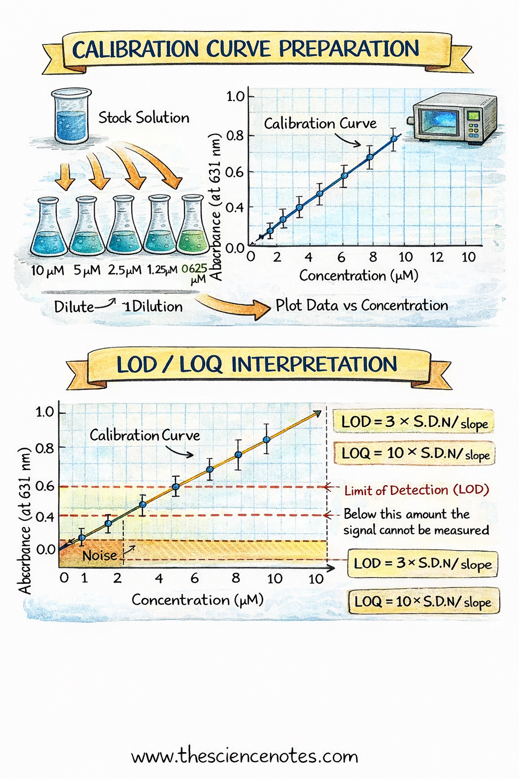
Limit of Detection (LOD): Minimum amount detectable above noise. Calculated as LOD = 3 × S.D./m.
Limit of Quantitation (LOQ): Minimum amount measurable with acceptable precision. LOQ = 10 × S.D./m.
Procedure: Preparing a Calibration Curve
1. Making Standards Using Serial Dilutions
Prepare a concentrated stock solution by accurately weighing the analyte and dissolving it in solvent.
Perform serial dilutions to generate a series of lower concentrations:
Dilute the stock solution stepwise into volumetric flasks.
Keep the dilution factor constant (e.g., 10-fold dilutions).
At least 5 concentrations are recommended for a reliable curve.
Note: Any pipetting errors propagate through serial dilutions, so careful technique is critical.
2. Measuring Instrumental Response
Measure the response of each standard using a suitable instrument (e.g., UV-Vis spectrophotometer, ion-selective electrode).
Take multiple readings (3–5 repeats) to estimate noise and improve accuracy.
Measure the unknown sample under identical conditions as the standards.
3. Plotting the Calibration Curve
Enter concentration vs. signal data into a spreadsheet.
Include error bars if repeated measurements were taken.
Fit the data to a linear or known non-linear function.
Use linear regression to calculate slope (m), intercept (b), and R².
Identify the linear portion and exclude outlier points only at the edges, not in the middle of the curve.
4. Calculating Unknown Concentration, LOD, and LOQ
Use the calibration curve equation to determine the unknown concentration.
Calculate LOD and LOQ using the slope and standard deviation of noise.
Dilute samples if they exceed the linear range of the instrument.
Example: UV-Vis Calibration of Blue Dye #1
Measured absorbance of 0–10 µM blue dye at 631 nm.
Linear regression gave: y = 0.109x + 0.0286, R² > 0.99.
Noise standard deviation: 0.021
LOD = 0.58 µM, LOQ = 1.93 µM
Unknown sample absorbance = 0.243 → concentration = 2.02 µM (before dilution correction)
Applications of Calibration Curves
Calibration curves are widely used across various fields:
Environmental Analysis: Determining pollutants in water or soil samples.
Biochemistry: Measuring neurotransmitters or proteins in biological fluids.
Pharmaceuticals: Quantifying vitamins, drugs, or additives.
Food Science: Analyzing caffeine, dyes, or nutrients in beverages and food.
Electrochemistry: Using ion-selective electrodes to quantify ions (e.g., fluoride) with log-scale calibration curves following the Nernst equation.
Tips for Accurate Calibration
Use a matrix that closely resembles the unknown sample.
Perform multiple measurements for each concentration to estimate noise.
Ensure concentrations bracket the expected range of unknowns.
Handle pipettes, balances, and volumetric flasks carefully to reduce error propagation.
Use software for plotting, regression, and error analysis.
Conclusion
Calibration curves are foundational in analytical chemistry. They enable researchers to predict unknown concentrations, calculate detection limits, and evaluate instrument sensitivity. By carefully preparing standards, running accurate measurements, and analyzing data correctly, calibration curves become a reliable tool for environmental, biological, pharmaceutical, and food science applications.